brainconn: a R-package for plotting brain connectivity data
Source:vignettes/brainconn.Rmd
brainconn.Rmd
Basic use of brainconn()
The brainconn() function allows users to input a binary/weighted and directed/directed (i.e. symmetric) connectivity matrix which can be plotted in MNI space onto several brain atlases provided with the package, or a user defined custom atlas. The layout of the nodes and edges is created using ggraph, which does most of the heavy lifting here. The background is a custom_annotation using ggplot2.
The minimum user input requirements for the brainconn() function is a connectivity matrix. This can be read into r as a matrix or data.fame. Some example connectivity matrices can be found in the data/example folder. The number of rows & columns should match the number of regions in the selected atlas. Custom atlases can also be used, see Using custom atlases.
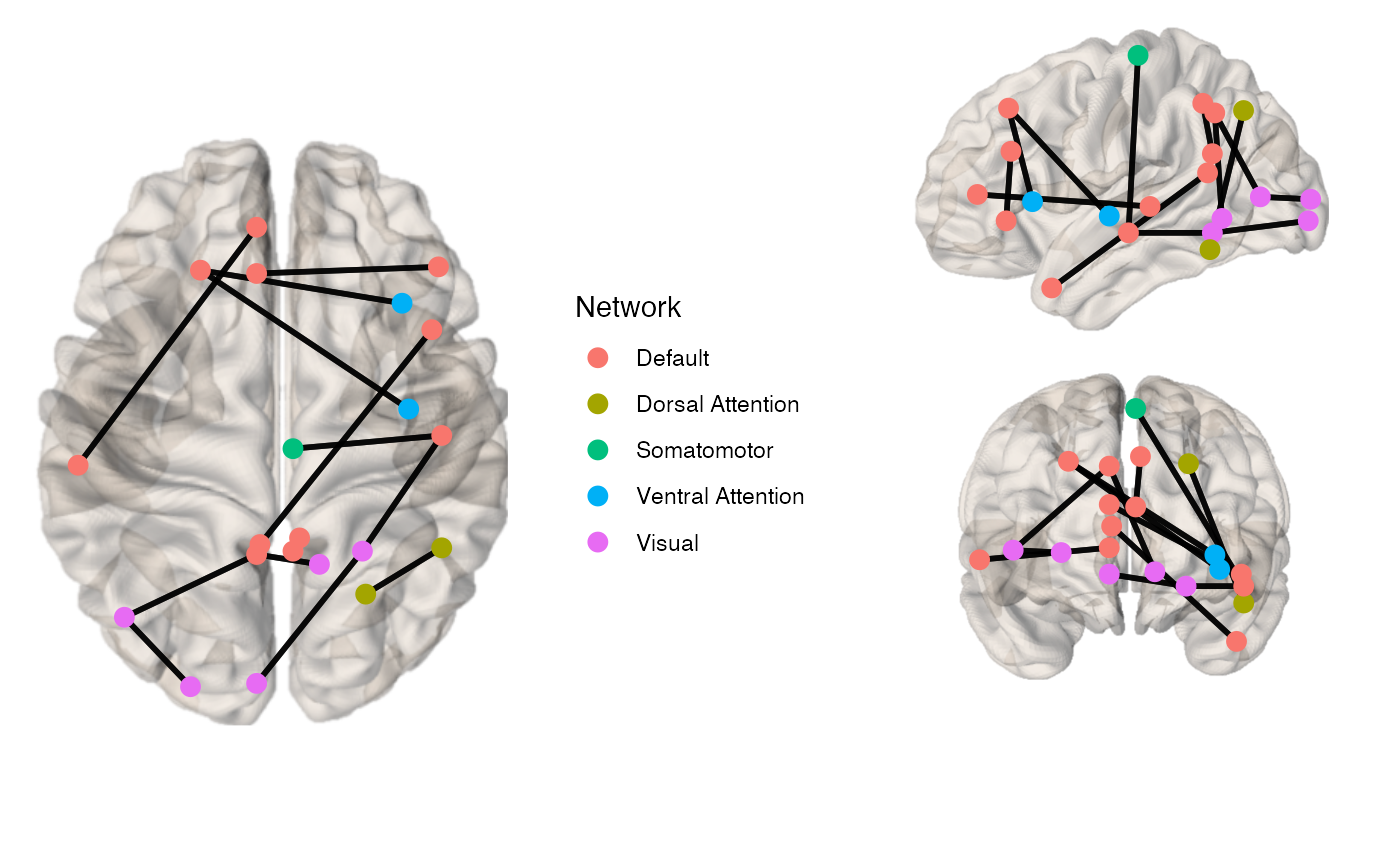
By default, the view is a top view, the node.color is by network.
library(brainconn) x <- example_unweighted_undirected brainconn(atlas ="schaefer300_n7", conmat=x, node.size = 3, view="ortho")
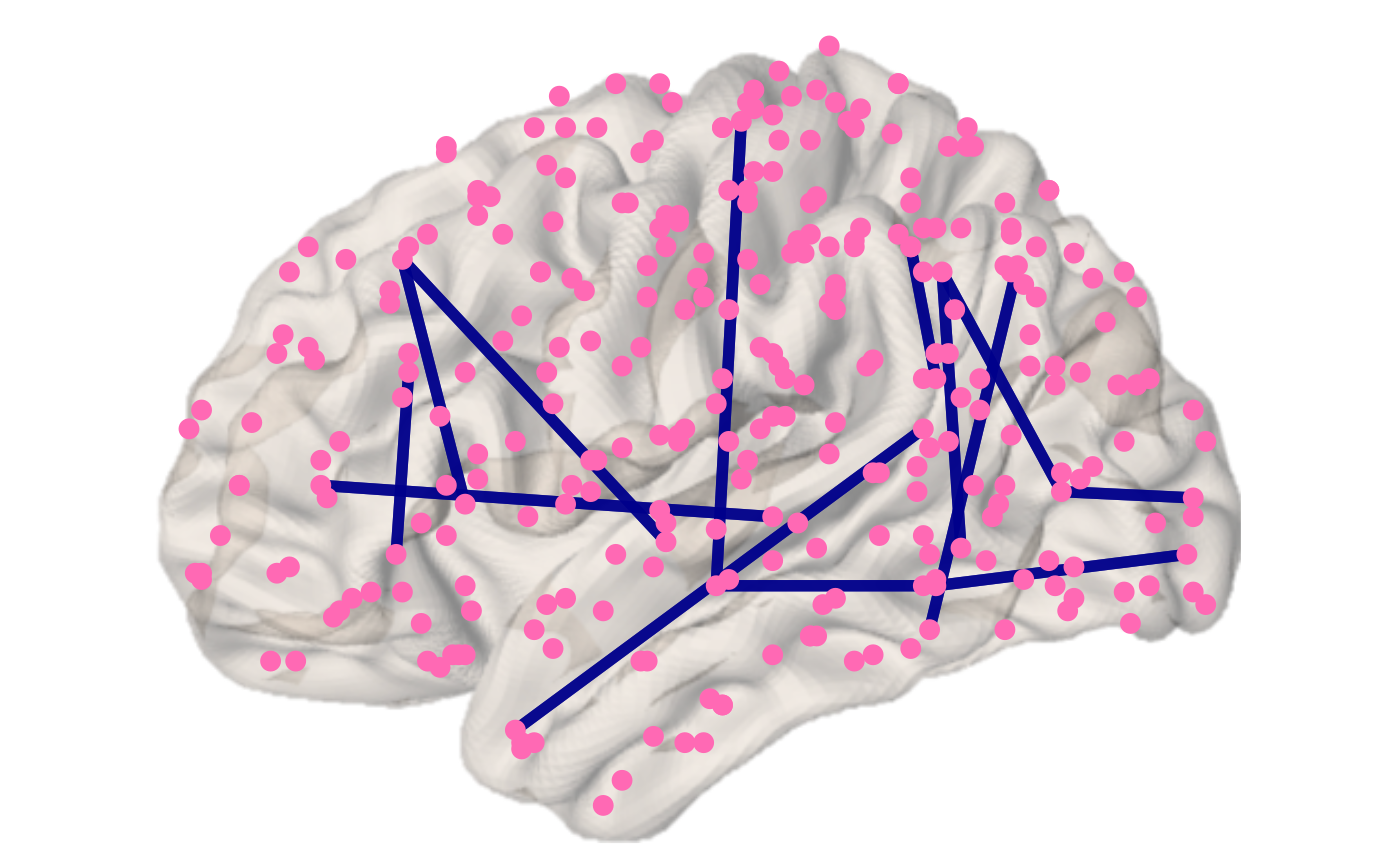
You can change the default view, node, edge and background properties as well as show all nodes of the atlas, rather than just the ones that have connected edges.
brainconn(atlas ="schaefer300_n7", conmat=example_unweighted_undirected, view="left", node.size = 3, node.color = "hotpink", edge.width = 2, edge.color="darkblue", edge.alpha = 0.8, all.nodes = T, show.legend = F)
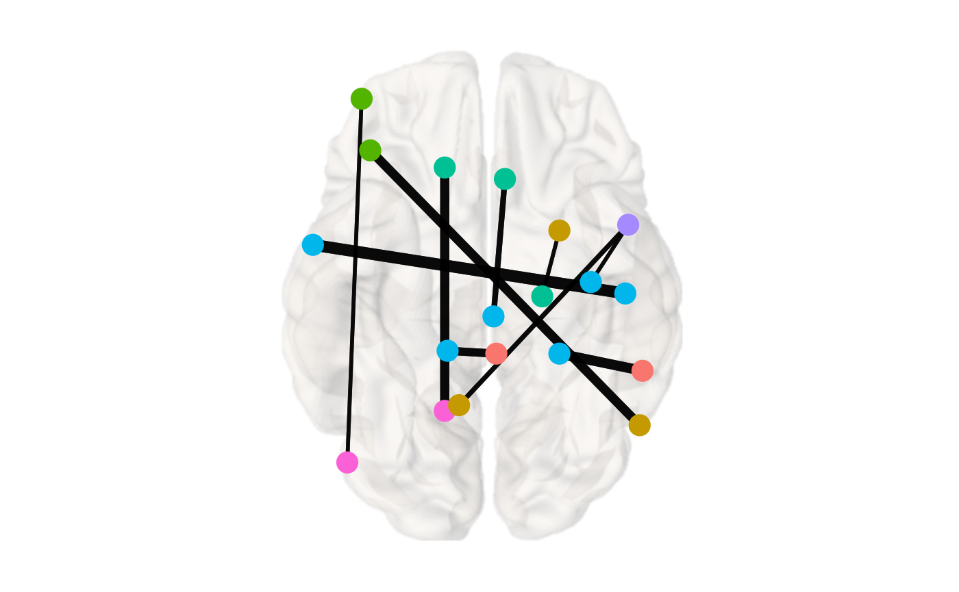
If the connectivity matrix you input is not a binary matrix, i.e. the values are weighted, by default braincon() will modulate the edge.width by the weighted values. scale.edge.width can be used to scale the edge width.
x <- example_weighted_undirected brainconn(atlas ="schaefer300_n7", conmat=x, node.size = 5,view="bottom", scale.edge.width = c(1,3), background.alpha = 0.4, show.legend = F)
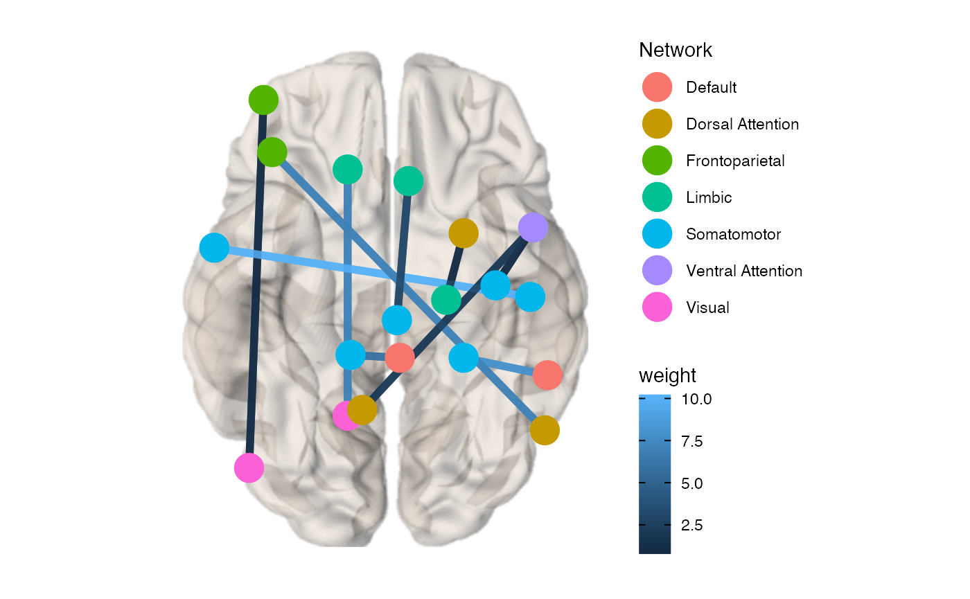
You can also color the edges by weight using the edge.color.weighted option.
brainconn(atlas ="schaefer300_n7", conmat=example_weighted_undirected, node.size = 7,view="bottom", edge.width = 2, edge.color.weighted = T, show.legend = T)
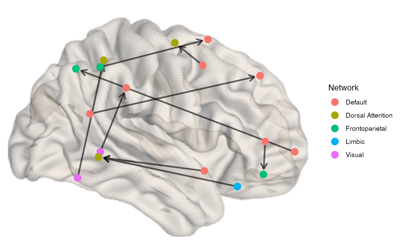
If the input is a directed matrix (i.e. non-symmetrical), the edges will be displayed as directed arrows, with the edge.width and edge.color serving the same purpose:
x <- example_unweighted_directed brainconn(atlas ="schaefer300_n7", conmat=x, node.size = 4, view="right", edge.alpha = 0.6)
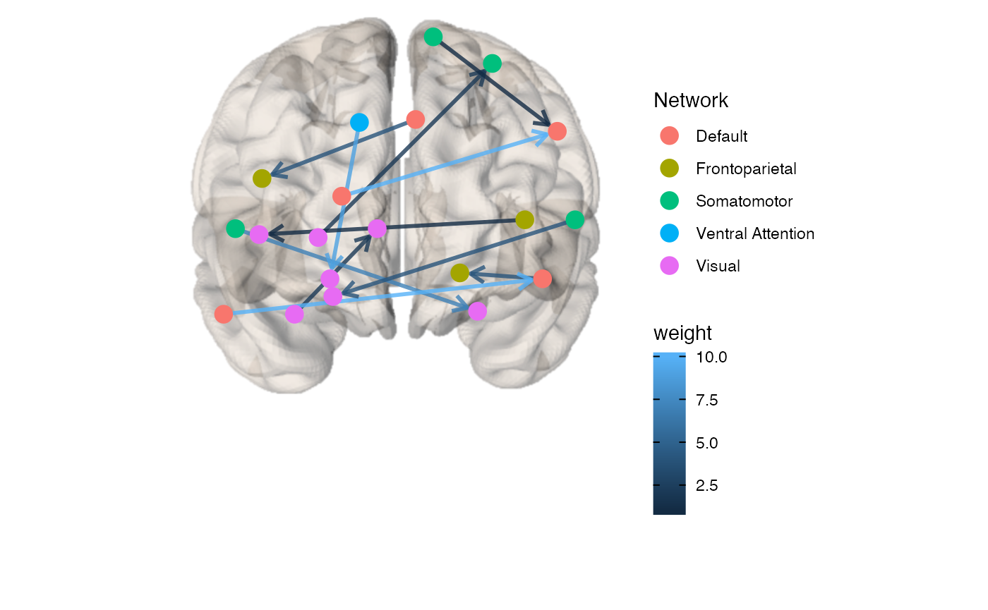
Weighted and directed matrix example:
x <- example_weighted_directed brainconn(atlas ="schaefer300_n7", conmat=x, view="front", edge.color.weighted=T)
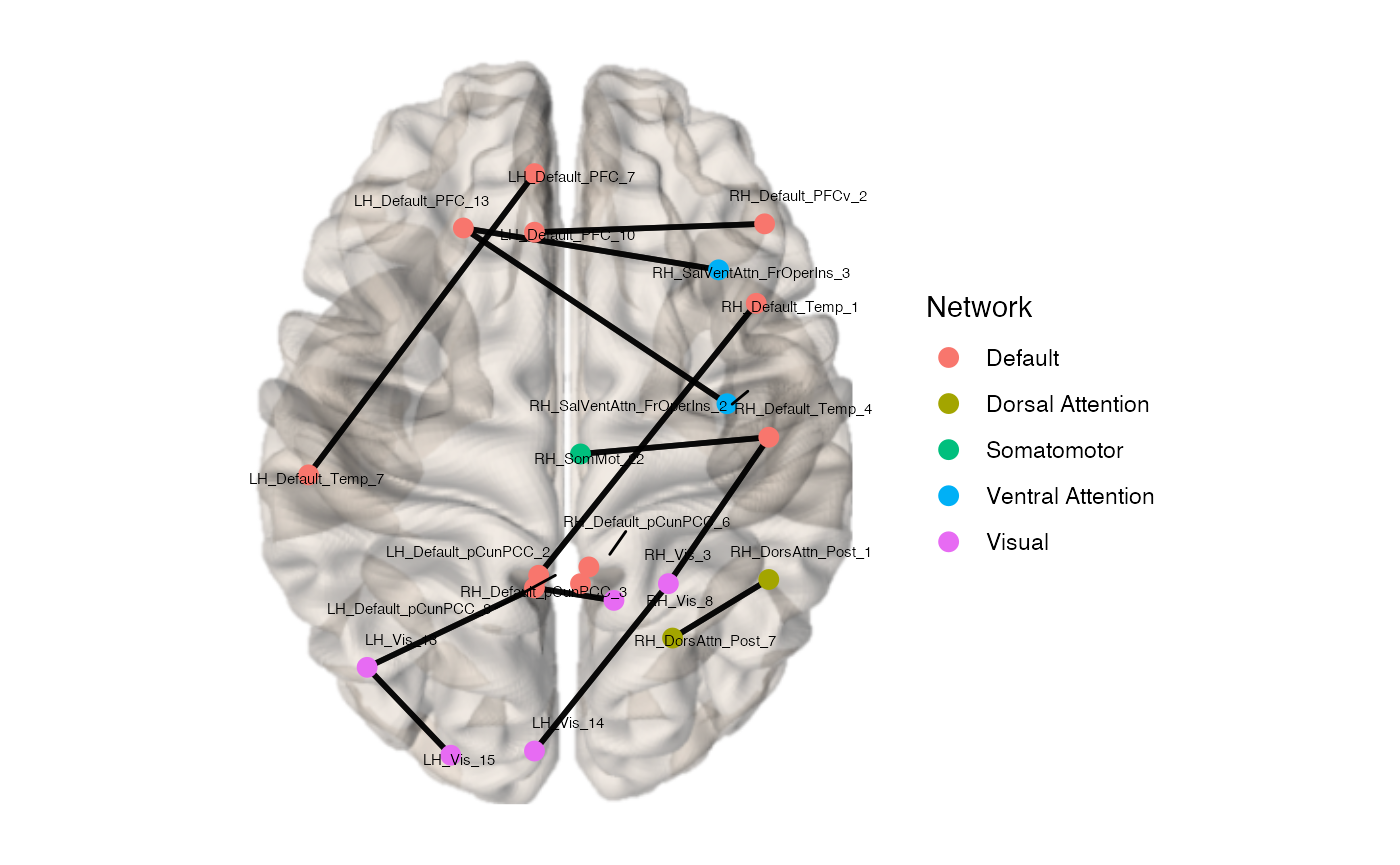
You can auto add labels, but this doesn’t work to great if theirs a large number of edges.
brainconn(atlas ="schaefer300_n7", conmat=example_unweighted_undirected, labels = T, label.size = 2, node.size = 3)
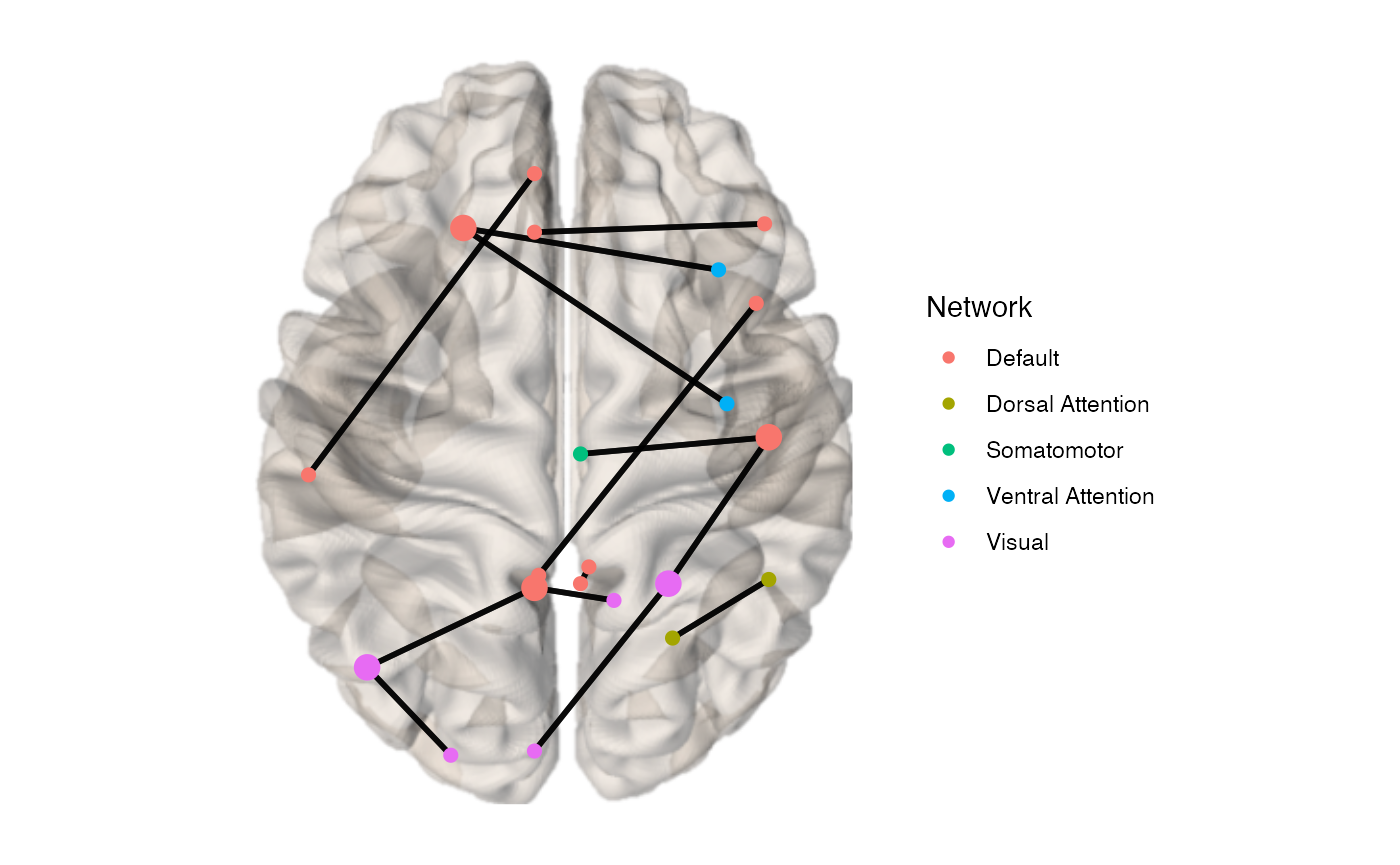
If you want to weight the nodes by a feature such as degree, you can provide a vector the length of the number of ROIs in the parcellation to node.size:
x <- example_unweighted_undirected x_igraph <- igraph::graph_from_adjacency_matrix(as.matrix(example_unweighted_undirected)) #convert connectivity matrix into an graph object. d <- igraph::degree(x_igraph) #use igraph::degree to obtain a vector of nodal degree d <- d[d != 0] #remove nodes with no edges brainconn(atlas ="schaefer300_n7", conmat=x, node.size = d)
Basic use of brainconn3D()
Currently, brainconn3D() is only able to visualize binary undirected connectivity matrices.
p <- brainconn3D(atlas ="schaefer300_n7", conmat=example_unweighted_undirected, show.legend = F) p